Example: Root Locus Design Method for DC Motor Speed
Control
Drawing
the open-loop root locus
Finding
the gain using the rlocfind command
Adding
a lag controller
Plotting
the closed-loop response
From the main problem, the dynamic equations and the open-loop transfer
function of DC Motor Speed are:


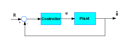
and the system schematic looks like:

With a 1 rad/sec step reference, the design criteria are:
- Settling time less than 2 seconds
- Overshoot less than 5%
- Steady-state error less than 1%
Now let's design a controller using the root locus method.
Create a new m-file and
type in the following commands (refer to main problem for the details of getting
those commands).
J=0.01;
b=0.1;
K=0.01;
R=1;
L=0.5;
num=K;
den=[(J*L) ((J*R)+(L*b)) ((b*R)+K^2)];
Drawing the open-loop root locus
The main idea of root locus design is to find the closed-loop response from
the open-loop root locus plot. Then by adding zeros and/or poles to the original
plant, the closed-loop response can be modified. Let's first view the root locus
for the plant. Add the following commands at the end of your m-file.
rlocus(num,den)
sgrid(.8,0)
sigrid(2.3)
title('Root Locus without a controller')
The command sigrid is the user-defined
function. You need to copy the sigrid.m file
to your directly before using it.
Two arguments in the sgrid command are the damping
ratio (zeta) term (0.8 corresponds to a overshoot of 5%), and the natural
frequency (Wn) term (= 0 corresponds to no rise time criterion) respectively.
The single argument in the sigrid command is the sigma term (4.6/2 seconds =
2.3). After you have saved sigma.m file to your
directly, run the above m-file in the command window. You should get the root
locus plot shown below:

Finding the gain using the rlocfind command
If you recall, we need the settling time and the overshoot to be as small as
possible. Large damping corresponds to points on the root locus near the real
axis. A fast response corresponds to points on the root locus far to the left of
the imaginary axis. To find the gain corresponding to a point on the root locus,
we can use the rlocfind command. We can find the gain and
plot the step response using this gain all at once. To do this, enter the
following commands at the end of your m-file and rerun it.
[k,poles] = rlocfind(num,den)
[numc,denc]=cloop(k*num,den,-1);
t=0:0.01:3;
step(numc,denc,t)
title('Step response with gain')
Go to the plot and select a point on the root locus half-way between
the real axis and the damping requirement, say at -6+2.5i. Matlab should return
the output similar to the following.
selected_point =
  -5.9596 + 2.0513i

k =
   10.0934

poles =
  -6.0000 + 2.0511i
  -6.0000 - 2.0511i
Note that the values returned in your Matlab command window may
not be exactly the same, but should at least have the same order of magnitude.
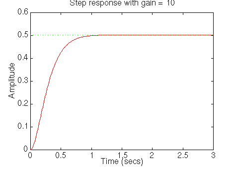
You should also get the following plot:

As you can see, the system is overdamped and the settling time is about one
second, so the overshoot and settling time requirements are satisfied. The only
problem we can see from this plot is the steady- state
error of about 50%. If we increase the gain to reduce the steady-state
error, the overshoot becomes too large (Try this yourself). We need to add a lag
controller to reduce the steady-state error.
Adding a lag controller
From the plot we see that this is a very simple root locus. The damping and
settling time criteria were met with the proportional controller. The
steady-state error is the only criterion not met with the proportional
controller. A lag
compensator can reduce the steady-state error. By doing this, we might
however increase our settling time. Try the following lag controller first:

This can be done by changing your m-file to look like the following:
J=0.01;
b=0.1;
K=0.01;
R=1;
L=0.5;
num=K;
den=[(J*L) ((J*R)+(L*b)) ((b*R)+K^2)];

z1=1;
p1=0.01;
numa = [1 z1];
dena = [1 p1];
numb=conv(num,numa);
denb=conv(den,dena);

rlocus(numb,denb)
sgrid(.8,0)
sigrid(2.3)
title('Root Locus with a lag controller')
numa and dena are the numerator and denominator of the
controller, and numb and denb are the numerator and denominator of
the overall open-loop transfer function.
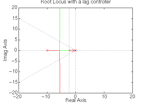
You should get the following root locus, which looks very similar to the
original one:

Plotting the closed-loop response
Now let's close the loop and see the closed-loop step response Enter the
following code at the end of your m-file:
[k,poles]=rlocfind(numb,denb)
[numc,denc]=cloop(k*numb,denb,-1);
t=0:0.01:3;
step(numc,denc,t)
title('Step response with a lag controller')
Rerun this m-file in the Matlab command window. When prompted to
select a point, pick one that is near the damping requirement (diagonal dotted
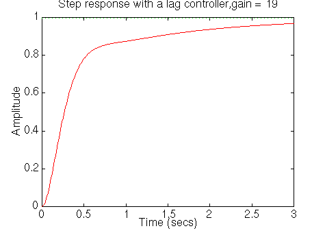
line). You should get the a plot similar to the following:

Your gain should be about 20. As you can see the response is not quite
satisfactory. You may also note that even though the gain was selected to
correlate with a position close to the damping criterion, the overshoot is not
even close to five percent. This is due to the effect of the lag controller
kicking in at a later time than the plant. (its pole is slower). What this means
is that we can go beyond the dotted lines that represent the limit, and get the
higher gains without worrying about the overshoot . Rerun your m-file, place the
gain just above the white, dotted line. Keep trying until you get a satisfactory
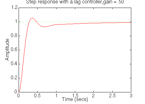
response. It should look similar to the following (we used a gain of around 50):

The steady-state error is smaller than 1%, and the settling time and
overshoot requirements have been met. As you can see, the design process for
root locus is very much a trial and error process. That is why it is nice to
plot the root locus, pick the gain, and plot the response all in one step. If we
had not been able to get a satisfactory response by choosing the gains, we could
have tried a different lag controller, or even added a lead controller.
[ Table des matičres ]


