Example: Frequency Design Method for DC Motor Speed
Control
Drawing
the original Bode plot
Adding
proportional gain
Plotting
the closed-loop response
Adding
a lag controller
From the main problem, the dynamic equations and the open-loop transfer
function of DC Motor Speed are:


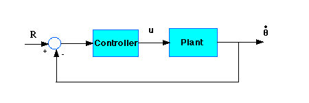
and the system schematic looks like:

With the 1 rad/sec step input, the design criteria are:
- Settling time less than 2 seconds
- Overshoot less than 5%
- Steady-state error less than 1%
Create a new m-file and
type in the following commands (refer to the main problem for the details of
getting those commands).
J=0.01;
b=0.1;
K=0.01;
R=1;
L=0.5;
num=K;
den=[(J*L) ((J*R)+(L*b)) ((b*R)+K^2)];
Drawing the original Bode plot
The main idea of frequency-based design is to use the Bode plot of the
open-loop transfer function to estimate the closed-loop response. Adding a
controller to the system changes the open-loop Bode plot, therefore changing the
closed-loop response. Let's first draw the Bode plot for the original open-loop
transfer function. Add the following code to the end of your m-file, and then
run it in the Matlab command window.
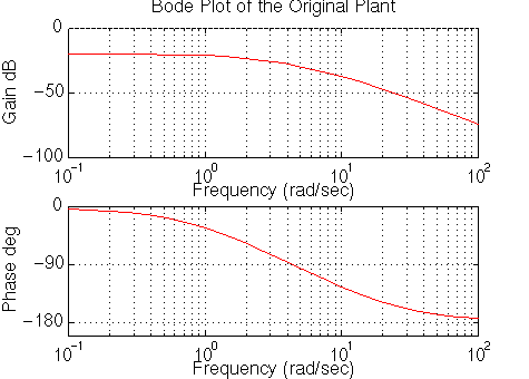
You should get the following
Bode plot:

Adding proportional gain
From the bode plot above, we see that the phase margin can be greater than
about 60 degrees if w is less than 10 rad/sec. Let's add gain to the system so
the bandwidth frequency is 10 rad/sec, which will give us a phase margin of
about 60 degrees. To find the gain at 10 rad/sec, you can try to read it off the
Bode plot (it looks to be slightly more than -40 dB, or 0.01 in magnitude). The
bode command, invoked with left-hand arguments, can also
be used to give you the exact magnitude:
[mag,phase,w] = bode(num,den,10)
mag =

    0.0139
To have a gain of 1 at 10 rad/sec, multiply the numerator by
1/0.0139 or approximately 72.
num = 70*num
and rerun your m-file. You should have the following Bode plot:

Plotting the closed-loop response
From the plot above we see that the phase margin is now quite large. Let's
see what the closed-loop response look like. Add a % in front of the
bode commands and add the following code to the
end of your m-file:
[numc,denc]=cloop(num, den, -1);
t=0:0.01:10;
step(numc,denc,t)
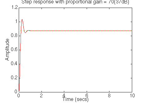
You will see the following plot:

The settling time is fast enough, but the overshoot and the steady-state
error are too high. The overshoot can be reduced by reducing the gain a bit
to get a higher phase margin, but this would cause the steady-state error to
increase. A lag controller is probably needed.
Adding a lag controller
We can add a lag
controller to reduce the steady-state error. At the same time, we should try
to reduce the overshoot by reducing the gain. Let's reduce the gain to 50, and
try a lag controller of

which should reduce the steady-state error by a factor of 1/0.01 = 100 (but
could increase the settling time). Go back and change your m-file so it looks
like the following:
num=K;
den=[(J*L) ((J*R)+(L*b)) ((b*R)+K^2)];
num=50*K;

z=1;
p=0.1;
numa=[1 z];
dena=[1 p];
numb=conv(num,numa);
denb=conv(den,dena);

bode(numb,denb)
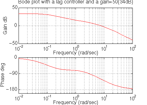
Rerun the file and you will get this plot:

The phase margin looks good. The steady-state error is predicted to be about
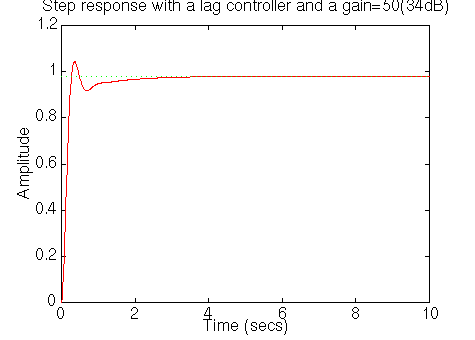
1/40dB or 1%, as desired. Close the loop and look at the step response. Add the
following lines of code to the end of you m-file and rerun.
[numc,denc]=cloop(numb, denb, -1);
t=0:0.01:10;
step(numc,denc,t)

Now you have a step response that meets the design requirements. The
steady-state error is less than 1%, the overshoot is about 5%, and the settling
time is about 2 seconds.
[ Table des matičres ]


