Root Locus Design for DC Motor Position Control

Example: Root Locus Design Method for DC Motor Position Control

Drawing the open-loop root locus
Integral Control
Proportional plus Integral Control
Proportional plus Integral plus Derivative Control
Finding the gain using the rlocfind command and plotting the closed-loop response

From the main problem, the dynamic equations in transfer function form are the following:

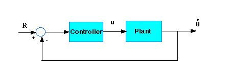
and the system schematic looks like:

With a 1 rad/sec step reference, the design criteria are:

Settling time less than 0.04 seconds
Overshoot less than 16%
No steady-state error
No steady-state error due to a disturbance

Now let's design a controller using the root locus method.

Create a new m-file and type in the following commands (refer to main problem for the details of getting those commands).

J=3.2284E-6;
b=3.5077E-6;
K=0.0274;
R=4;
L=2.75E-6;
num=K;
den=[(J*L) ((J*R)+(L*b)) ((b*R)+K^2) 0];

Drawing the open-loop root locus

The main idea of root locus design is to find the closed-loop response from the open-loop root locus plot. Then by adding zeros and/or poles to the original plant, the closed-loop response will be modified. Let's first view the root locus for the plant. Add the following commands at the end of your m-file.

rlocus(num,den)
sgrid(.5,0)
sigrid(100)

The commands sgrid and sigrid are functions. Sgrid is a function in the Matlab tool box, but sigrid is not. You need to copy the sigrid.m file to your directly. Click here to see how to copy sigrid.m into an m-file. The variables in the sgrid command are the zeta term (0.5 corresponds to a overshoot of 16%), and the wn term (no rise time criteria) respectively. The variable in the sigrid command is the sigma term (4/0.04 seconds = 100). Run the above m-file and you should get the root locus plot below:

If you look at the axis scales on this plot, one open-loop pole is very far to the left (further than -1x10^6). This pole does not affect the closed loop dynamics unless very large gains are used, where the system becomes unstable. We will ignore it by changing the axes to zoom in to just the lower-gain portion of the root locus. Add the following command to your m-file and re-run it.

axis([-400 100 -200 200])

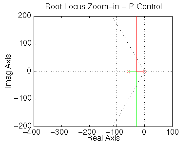
You should obtain the following plot in which you can see that the closed-loop system will be stable for small gains.

We can see from this plot that the closed-loop poles are never fast enough to meet the settling time requirement (that is, they never move to the left of the sigma=100 vertical line). Also, recall that we need an integrator in the controller (not just in the system) to remove steady-state error due to a disturbance.

Integral Control

Now, let's try using integral control to remove steady-state error to a disturbance. Modify your m-file so it looks like:

J=3.2284E-6;
b=3.5077E-6;
K=0.0274;
R=4;
L=2.75E-6;
num=K;
den=[(J*L) ((J*R)+(L*b)) ((b*R)+K^2) 0];

numcf=[1];
dencf=[1 0];
numf=conv(numcf,num);
denf=conv(dencf,den);
rlocus(numf,denf)
sgrid(.5,0)
sigrid(100)
axis([-400 100 -200 200])

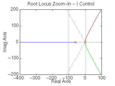
Note that this adds a 1/s term to the forward loop. In this m-file, we are ignoring the fast pole, and just zooming in to the low-gain portion of the root locus. Run this m-file and you will obtain the following plot.

From this root locus we can see that the closed-loop system under integral control is never stable, and another controller must be used.

Proportional plus Integral Control

Now, let's modify the integral controller to a PI controller. Using PI instead of I control adds a zero to the open-loop system. We'll place this zero at s=-20. The zero must lie between the open-loop poles of the system in this case so that the closed-loop will be stable. Change the lines defining the controller (numcf and dencf) in your m-file to the following.

numcf=[1 20];
dencf=[1 0];

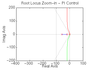
Re-run your m-file and obtain the following plot.

Now, we have managed to stabilize the system with zero steady-state error to a disturbance, but the system will still not be fast enough.

Proportional plus Integral plus Derivative Control

In order to pull the root locus further to the left, to make it faster, we need to place a second open-loop zero, resulting in a PID controller. After some experimentation, we can place the two PID zeros at s=-60 and s=-70. Change the lines defining the controller (numcf and dencf) in your m-file to the following.

numcf=conv([1 60],[1 70]);
dencf=[1 0];

Re-run your m-file and obtain the following plot.

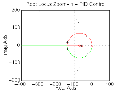
Now, we can see that two of the closed-loop poles loop around well within both the settling time and percent overshoot requirements. The third closed loop pole moves from the open-loop pole at s=-59.2 to the open loop zero at s=-60. This closed-loop pole nearly cancels with the zero (which remains in the closed loop transfer function) because it is so close. Therefore, we can ignore it's effect. However, the other open-loop zero also remains in the closed-loop, and will affect the response, slowing it down, and adding overshoot. Therefore, we have to be conservative in picking where on the root locus we want the closed-loop poles to lie.

Finding the gain using the rlocfind command

If you recall, we need the settling time and the overshoot to be as small as possible, particularly because of the effect of the extra zero. Large damping corresponds to points on the root locus near the real axis. A fast response corresponds to points on the root locus far to the left of the imaginary axis. To find the gain corresponding to a point on the root locus, we can use the rlocfind command. We can find the gain and plot the step response using this gain all at once. To do this, enter the following commands at the end of your m-file and rerun it.

 
[k,poles] = rlocfind(numf,denf)
[numc,denc]=cloop(k*numf,denf,-1); 
t=0:0.001:.1; 
step(numc,denc,t)

Go to the plot and select a point on the root locus on left side of the loop, close to the real axis as shown below with the small black + marks. This will ensure that the response will be as fast as possible with as little overshoot as possible. These pole locations would indicate that the response would have almost no overshoot, but you must remember that the zero will add some overshoot.

After doing this, you should see the following output in the Matlab command window.

 
selected_point =

 -1.3943e+02+  1.8502e+01i


k =

    0.1309


poles =

   1.0e+06 *

  -1.4542          
  -0.0001 + 0.0000i
  -0.0001 - 0.0000i
  -0.0001

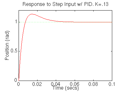
Note that the values returned in your Matlab command window may not be exactly the same, but should at least have the same order of magnitude. You should also get the following step response plot:

As you can see, the system has an overshoot of approximately 15%, a settling time of approximately 0.04 seconds, and no steady-state error.

Let's now look at the disturbance response by computing the closed-loop disturbance transfer function and plotting its step response. Add the following lines to your m-file:

numdcl=conv(numc,dencf);
dendcl=conv(denc,numcf);
step(numdcl,dendcl,t);

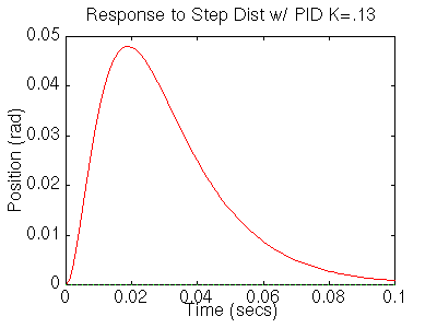
Re-run your m-file, selecting the same point on the root locus, and you will get the following plot.

You can see that the disturbance reaches a steady-state value of zero, and in fact, stays within 0.02 (or 2%) afte 0.04 seconds. Therefore, all the design requirements have been met.

In this example, we placed zeros on the root locus to shape it the way we wanted. While some trial-and error is necessary to place the zeros, it is helpful to understand how the root locus is drawn, and Matlab is used to verify and refine the placement.

[ Table des matières ]