Example: Frequency Design Method for DC Motor Position
Control
Drawing
the original Bode plot
Adding
an integrator
Gain
and phase margin specification and controller design
From the main problem, the dynamic equations in transfer-function form are
the following:


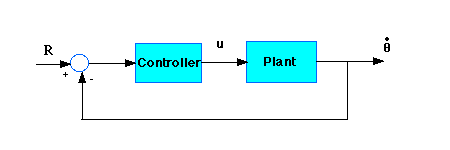
and the system schematic looks like:

With a 1 rad/sec step reference, the design criteria are:
- Settling time less than 40 milliseconds
- Overshoot less than 16%
- No steady-state error
- No steady-state error due to a step disturbance
Drawing the original Bode plot
Create a new m-file and
type in the following commands.
J=3.2284E-6;
b=3.5077E-6;
K=0.0274;
R=4;
L=2.75E-6;
num=K;
den=[(J*L) ((J*R)+(L*b)) ((b*R)+K^2) 0];
The main idea of frequency-based design is to use the Bode plot of
the open-loop transfer function to estimate the closed-loop response. Adding a
controller to the system changes the open-loop Bode plot, therefore changing the
closed-loop response. Let's first draw the Bode plot for the original open-loop
transfer function. Add the following code to the end of your m-file, and then
run the m-file.
w=logspace(0,4,101);
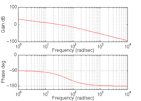
bode(num,den,w)
You should get the following Bode plot:

Adding an integrator
Now lets add an integrator for zero steady-state error in response to a step
disturbance. Add the following lines to your m-file:
numi=1;
deni=[1 0];
numiol=conv(num,numi);
deniol=conv(den,deni);
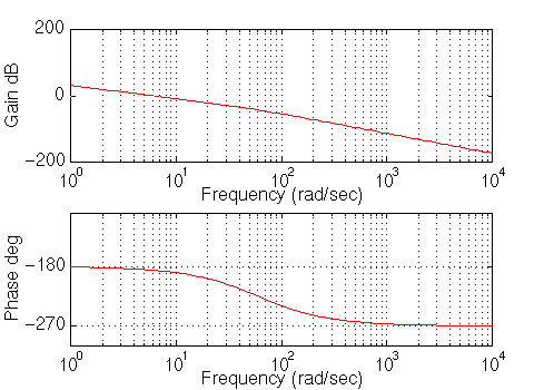
bode(numiol,deniol,w)
You should get the following plot:

Gain and Phase Margin Specifications and Controller Design
We want less than a 16% overshoot, so lets compute the damping ratio based on
a 16% overshoot. Also the corresponding phase margin is 100 times the damping
ratio. From the settling time requirement, we are able to compute the desired
bandwidth frequency. Add the following lines to your m-file:
zeta=-log(.16)/sqrt(pi^2+(log(.16))^2);
PM=100*zeta;
wbw=(4/(0.04*zeta))*sqrt((1-2*zeta^2)+sqrt(4*zeta^4-4*zeta^2+2));
We want to have at least 50 degrees of phase margin, therefore the
gain should fall between -6 and -7.5 dB at some frequency after 250 rad/sec.
From the Bode plot we see that we must add about 80 degrees of phase and 60 dB
of gain at a frequency of 250 rad/sec. The gain plot will then lie between -6
and -7.5 dB and after 244 rad/sec. From the Bode phase plot we can see that
there is a pole near 60 rad/sec. We will use a PI controller to put a zero at
s=60 to flatten out the phase curve. Add the following lines to your m-file:
numpi=[1 60];
denpi=[1 0];
numpiol=conv(numpi,num);
denpiol=conv(denpi,den);
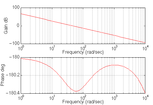
bode(numpiol,denpiol,w)
You should see the following plot:

From the bode plot we can see that we need 50 more degrees of phase at a
frequency of 250 rad/sec. Lets now try a lead compensator to add exactly 50
degrees of phase. Add the following lines to your m-file:
a=(1 - sin(PM*pi/180))/(1 + sin(PM*pi/180));
T=1/(wbw*sqrt(a));
numpil = conv([1 60],[T 1]);
denpil = conv([1 0],[a*T 1]);
numpilol = conv(numpil,num);
denpilol = conv(denpil,den);
w = logspace(2,3,101);
bode(numpilol,denpilol,w)

This new Bode plot now shows that the phase margin is about right at 250
rad/sec, but the gain is too small by about 20 dB. The gain crossover must occur
at 240 rad/sec. To bring the gain up by 20 dB we will multiply by a gain of 10.
Add the following lines to your m-file:
kpid = 10;
bode(kpid*numpilol,denpilol,w)
You should get the following plot:

Lets now check the step response of the closed loop system. Add the following
lines to youe m-file:
[numpilcl,denpilcl] = cloop(kpid*numpilol,denpilol,-1);
t = 0:0.001:0.1;
step(numpilcl,denpilcl)
You should get the following plot:

The overshoot is now too large, however the settling time is better than
expected. So let's try another design where the phase margin is larger, say
around 70 degrees. Add the following lines to your m-file:
PM=70;
a=(1 - sin(PM*pi/180))/(1 + sin(PM*pi/180));
T=1/(wbw*sqrt(a));
numpil=conv([1 60],[T 1]);
denpil=conv([1 0],[a*T 1]);
numpilol=conv(numpil,num);
denpilol=conv(denpil,den);
w=logspace(2,3,101);
bode(numpilol,denpilol,w)
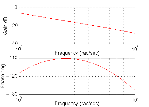
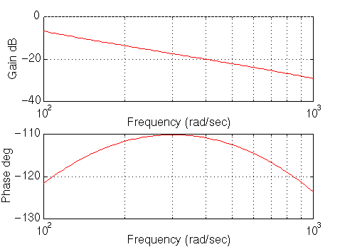
You should get the following plot:

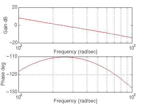
This new bode plot shows that the phase margin is good at around 250 rad/sec,
but the gain is too small by about 14 dB. The gain crossover must occur at 240
rad/sec. To bring the gain up we will multiply by a gain of 5. Add the following
lines to your m-file:
kpid = 5;
bode(kpid*numpilol,denpilol,w)
You should get the following plot:

Now lets check the step response again. Add the following lines to your
m-file:
[numpilcl,denpilcl] = cloop(kpid*numpilol,denpilol,-1);
t = 0:0.001:0.1;
step(numpilcl,denpilcl)
You should get the following step response:

From the step response we now see that the overshoot is fine, but the
settling time is too long. Let's try a slightly higher bandwidth. Add the
following lines to your m-file:
wbw=300;
a=(1-sin(PM*pi/180))/(1+sin(PM*pi/180));
T=1/(wbw*sqrt(a));
numpil=conv([1 60],[T 1]);
denpil=conv([1 0],[a*T 1]);
numpilol=conv(numpil,num);
denpilol=conv(denpil,den);
w=logspace(2,3,101);
bode(numpilol,denpilol,w)
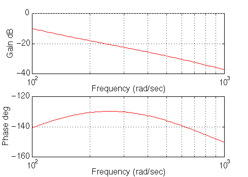
You should get the following plot:

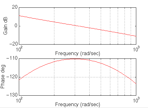
This new bode plot shows that the phase margin is about right at a frequency
of 250 rad/sec, but the gain is too small by about 18 dB. The gain crossover
must occur at 240 rad/sec. To bring the gain up we will multiply by a gain of 8.
Add the following lines to your m-file:
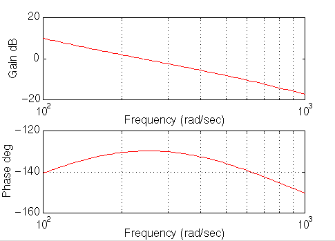
kpid=8;
bode(kpid*numpilol,denpilol,w);
You should get the following plot:

Now let's check the step response of the closed loop system. Add the
following lines to your m-file:
[numpilcl,denpilcl]=cloop(kpid*numpilol,denpilol,-1);
t=0:0.001:0.1;
step(numpilcl,denpilcl)
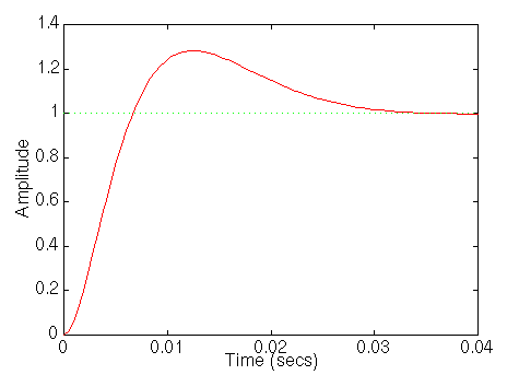
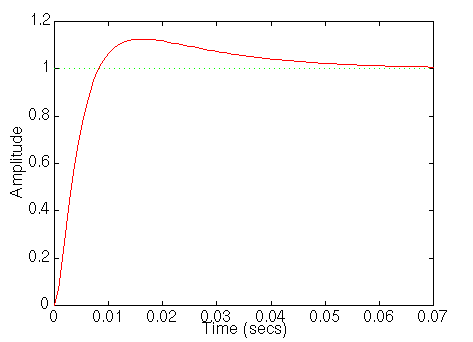
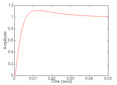
You should get the following step response:

Now everything looks good. We have less than 16% overshoot and a settling
time of about 40 milliseconds.
Note: As you noticed, the frequency response method
for this particular problem requires substantial amount of trial and error runs.
The m-file below is the simplified version of what was done above. After you run
this m-file, you will get the last two plots shown above.
J=3.2284E-6;
b=3.5077E-6;
K=0.0274;
R=4;
L=2.75E-6;
num=K;
den=[(J*L) ((J*R)+(L*b)) ((b*R)+K^2) 0];
PM=70;
wbw=300;
a=(1-sin(PM*pi/180))/(1+sin(PM*pi/180));
T=1/(wbw*sqrt(a));
numpil=conv([1 60],[T 1]);
denpil=conv([1 0],[a*T 1]);
numpilol=conv(numpil,num);
denpilol=conv(denpil,den);
kpid=8;
w=logspace(2,3,101);
bode(kpid*numpilol,denpilol,w)
figure
[numpilcl,denpilcl]=cloop(kpid*numpilol,denpilol,-1);
t=0:0.001:0.1;
step(numpilcl,denpilcl)
[ Table des matičres ]


