Control design using pole placement
Reference input
The state equations for this problem are:

where
- m=1000 kg
- b=50 N*sec/kg
- u=500 N
- v=velocity
- y=output
The design criteria are:
Overshoot < 10%
Steady state error < 2%
where
We should use the technique called "pole placement" to obtain
the desired output. Poles of a closed-loop system can be found from the
characteristic equation: the determinate of [sI-(A-B*K)] matrix. If desired
poles can be placed into the system by designing right control matrix (K), then
the desired output can be obtained. In this tutorial, poles will be chosen
first, then use Matlab to find the corresponding control matrix (K).
Now, we need to determine where to place poles for our system. Since our
[sI-(A-B*K)] matrix is 1x1, we have only one pole to place. Let the pole to be
at -1.5 (arbitrary). Just as in the State-Space Tutorial, the Matlab function
called place will be used to find
the control matrix K . Create an new m-file and
enter the following commands.
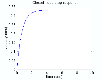
As you can see, the rise time is satisfactory, but the steady-state error is
too large.
Scaling factor called Nbar (the schematic is shown below)
should be used to eliminate the steady-state error. Unlike the example in the
Tutorial, the command rscale is not
applicable for our system. Nbar needs to be determined manually.
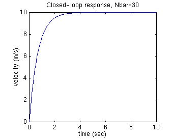
After several trial-and-error runs, the Nbar equals 30 provided the desired
step response. Copy the following commands to an m-file and run it in the Matlab
command window. You should get the step response shown below.
As you can see, the steady-state error has been eliminated. The rise time is
less than 5 seconds and the overshoot is, in fact, zero. All the design
requirements are satisfied.
Control design using pole placement
The schematic of a full-state
feedback system is shown below.

m=1000;
b=50;
t=0:0.1:10;
u=500*ones(size(t));
A=[-b/m];
B=[1/m];
C=[1];
D=[0];
x0=[0];
p1=-1.5;
K=place(A,B,[p1])
A1=A-B*K;
lsim(A1,B,C,D,u,t,x0);
Running this m-file in the Matlab command window should give you the
control matrix and the following step response.

Reference input

m=1000;
b=50;
t=0:0.1:10;
u=500*ones(size(t));
A=[-b/m];
B=[1/m];
C=[1];
D=[0];
x0=[0];
p1=-1.5
K=place(A,B,[p1]);
Nbar=30;
A1=A-B*K;
lsim(A1,B*Nbar,C,D,u,t,x0);
